Intro to Jax
Imports
Some of the libraries we will use throughout this post are imported below.
import time

import numpy as np
import matplotlib.pyplot as plt
import matplotlib as mpl
import seaborn as sns
Introduction
The Jax Quickstart tutorial states
JAX is NumPy on the CPU, GPU, and TPU, with great automatic differentiation for high-performance machine learning research.
What does this mean? And how does this differ from other deep learning libraries such as torch and tensorflow?
As is standard we will import some jax libraries and functions
import jax
from jax import jit, grad, vmap
from jax import random
import jax.numpy as jnp
import jax.scipy as jscp
Backend: XLA
Jax is basically a compiler for turning python code and vector operations using the XLA compiler to machine instructions for different computer architectures. The standard computer architecture we use is the GPU, but there are others, for example
or other specially created hardware which accelerates operations or make them more efficient in some way. The point is that python is slow and XLA makes this very fast using techniques such as fusing operations and removing redundant code and operations. Personally, this feels like a pretty future-proof way of decoupling how we specify what we want using e.g. python+jax vs how it is made to run on hardware, here using XLA. It reminds me of how LSP has solved the decoupling problem for code editing for editors1. There seem to be even more specialized hardware being created for e.g. inference of LLMs (like this which is one of several LLM inference hardware companies I saw at NeurIPS 2023) so who knows what funky architectures will become available in the future.
What is jax?
Jax is a reimplementation of the older linear algebra and science stack for python including numpy and scipy, with a just-in-time compiler and ways to perform automatic differentiation. To really hammer this home, jax has reimplemented a subset of both of these packages which seem pretty feature-complete. The current state of this API can be found in the docs.
Jax primitives: jit, grad, vmap
There are 3 functions which are integral to almost any jax program.
jit
The jit function takes a large subset of python together with jax functions and compile it down to XLA-kernels which are very fast. Below I've done a very quick benchmark of how jit speeds up matrix-matrix multiplication.
def jax_matmul(A, B):
    A @ B

jit_jax_matmul = jit(jax_matmul)

import timeit
n, p, k = 10**4, 10**4, 10**4
A = jnp.ones((n, p))
B = jnp.ones((p, k))
jit_jax_matmul(A, B) # Trace the jit function once
print(f"jax: {timeit.timeit(lambda: jax_matmul(A, B).block_until_ready(), number=10)}")
print(f"jax (JIT): {timeit.timeit(lambda: jit_jax_matmul(A, B).block_until_ready(), number=10)}")
jax: 0.37372643800335936
jax (JIT): 0.0003170749987475574
which is about double the speed. The gains are much greater when we jit things which does not have an already efficient implementation (such as a matmul). Additionally, this allows us to speed things up which cannot be done without considerable vectorization effort in numpy or may be outright impossible.
grad
The grad function takes as input a function \(f\) mapping to \(\mathbb{R}\) and spits out the gradient of that function \(\nabla f\). This can be a very natural way of working with gradients if you are used to the math.
def sum_of_squares(x):
    return jnp.sum(x**2)

sum_of_squares_dx = grad(sum_of_squares)
The function sum_of_squares_dx is the mathematical gradient of sum_of_squares. The randomness is handled explicitly by splitting the state (key), read about it here.
key = jax.random.PRNGKey(0)
key, subkey = jax.random.split(key)
in_x = jax.random.normal(key, (3, 3))
dx = sum_of_squares_dx(in_x)
print(dx)
print(dx.shape)
[[-5.2211165   0.06770565  2.1726665 ]
 [-2.960598    3.0806496   2.125032  ]
 [ 1.0834967   0.0340456   0.544537  ]]
(3, 3)
vmap
The function vmap allows you to lift a function to a batched function, without having to go through vectorization. For example, if we wanted to batch the sum_of_squares function we can do this by simply applying vmap
batched_sum_of_squares = vmap(sum_of_squares)
x = jax.random.normal(key, (5, 3, 3))
print(batched_sum_of_squares(x))
print(batched_sum_of_squares(x).shape)
[ 7.109205   7.1214614 21.167786   6.137778   4.915494 ]
(5,)
This is pretty powerful: often it's easy to specify the function for a sample \(x\) but harder to vectorize. For a standard neural network it may be pretty simple, but imagine something like LLMs, GANs or working with inputs which are not points, e.g. sets. Additionally, we can use the in_axes argument to batch in according to different input arguments and ignore others.
def multi_matmul(A, B, C):
    return A @ B @ C

# Batch according to first and third input argument, not second
vmap_multi_matmul = vmap(multi_matmul, in_axes=(0, None, 0))

l, n, p, d, m = 3, 5, 7, 9, 11
A = jnp.ones((l, n, p))
B = jnp.ones((p, d))
C = jnp.ones((l, d, m))

print(vmap_multi_matmul(A, B, C).shape) # l batches of (n, m) -> (l, n, m)
(3, 5, 11)
Composition
You can compose all of these functions as you see fit
jit_batched_sum_of_squares_dx = jit(vmap(grad(sum_of_squares)))
print(jit_batched_sum_of_squares_dx(x).shape)
(5, 3, 3)
This allows for utlizing the autodiff framework fully.
Building a neural network from scratch
We'll build an MLP using nothing but jax. We will train this on MNIST. To load the data I'm using the jax-dataloader library.
import jax_dataloader as jdl
from torchvision.datasets import MNIST

pt_ds = MNIST("/tmp/mnist", download=True, transform=lambda x: np.array(x, np.float32), train=True)
train_dataloader = jdl.DataLoader(pt_ds, backend="pytorch", batch_size=128, shuffle=True)
pt_ds = MNIST("/tmp/mnist", download=True, transform=lambda x: np.array(x, np.float32), train=False)
test_dataloader = jdl.DataLoader(pt_ds, backend="pytorch", batch_size=128, shuffle=True)
The jax library have some helpful functions for building neural networks. Here we create parameters and define a prediction function which given a pytree of parameters and an input outputs the predicted logits. Pytrees is a great thing about jax where it allow us to intuitively and effectively use not only raw arrays but also tree-like structures of by composing lists, tuples and dictionaries with each other and arrays as leaves and map over these as if they were arrays.
Creating the neural network
from jax.nn import relu
from jax.nn.initializers import glorot_normal
from jax.scipy.special import logsumexp

def create_mlp_weights(num_layers: int, in_dim: int, out_dim: int, hidden_dim: int, key):
    # Create helper function for generating weights and biases in each layer
    def create_layer_weights(in_dim, out_dim, key):
        return {
            "W": glorot_normal()(key, (in_dim, out_dim)),
            "b": np.zeros(out_dim)
        }
    params = []
    key, subkey = jax.random.split(key)
    # Fill out parameter list with dictionary of layer-weights and biases
    params.append(create_layer_weights(in_dim, hidden_dim, subkey))
    for _ in range(1, num_layers):
        key, subkey = jax.random.split(key)
        params.append(create_layer_weights(hidden_dim, hidden_dim, key))
    key, subkey = jax.random.split(key)
    params.append(create_layer_weights(hidden_dim, out_dim, subkey))
    return params

def predict(params, x):
    for layer in params[:-1]:
        x = relu(x @ layer["W"] + layer["b"])
    logits = x @ params[-1]["W"] + params[-1]["b"]
    return logits - logsumexp(logits)
Let's pick some reasonable defaults. We see that all shapes are correct and we have batched the predict function.
num_layers = 3
in_dim = 28 * 28
out_dim = 10
hidden_dim = 128
key = jax.random.PRNGKey(2023)
params = create_mlp_weights(num_layers, in_dim, out_dim, hidden_dim, key)
print(predict(params, jnp.ones(28 * 28)))

batched_predict = vmap(predict, in_axes=(None, 0))
print(batched_predict(params, jnp.ones((4, 28 * 28))).shape)
print(len(params))
print(type(params[0]["W"]))
[-3.3419425 -1.4851335 -2.5466485 -3.1445212 -1.8924606 -2.5047162
 -2.622343  -2.6072748 -1.5674857 -3.5270252]
(4, 10)
4
<class 'jaxlib.xla_extension.ArrayImpl'>
Training
Now we write the helper functions to train this network. In particular we use the pytree functionality of jax to update the parameters which is a pytree since it's a list of dictionaries of arrays.
import jax.tree_util as tree_util

def one_hot(x, k, dtype=jnp.float32):
  """Create a one-hot encoding of x of size k."""
  return jnp.array(x[:, None] == jnp.arange(k), dtype)

@jit
def accuracy(params, images, targets):
  target_class = jnp.argmax(targets, axis=1)
  predicted_class = jnp.argmax(batched_predict(params, images), axis=1)
  return jnp.mean(predicted_class == target_class)

def loss(params, images, targets):
  preds = batched_predict(params, images)
  return -jnp.mean(preds * targets)

@jit
def update(params, x, y, step_size):
  grads = grad(loss)(params, x, y)
  return tree_util.tree_map(lambda w, g: w - step_size * g, params, grads)

EPOCHS = 10
STEP_SIZE = 10 ** -2
train_acc = []
train_loss = []
test_acc = []
test_loss = []

for epoch in range(EPOCHS):
  print('Epoch', epoch)
  for image, output in train_dataloader:
    image, output = jnp.array(image).reshape(-1, 28 * 28), one_hot(jnp.array(output), 10)
    train_acc.append(accuracy(params, image, output).item())
    train_loss.append(loss(params, image, output).item())
    params = update(params, image, output, STEP_SIZE)
  print(f'Train accuracy: {np.mean(train_acc):.3f}')
  print(f'Train loss: {np.mean(train_loss):.3f}')
  _test_acc = []
  _test_loss = []
  for image, output in test_dataloader:
    image, output = jnp.array(image).reshape(-1, 28 * 28), one_hot(jnp.array(output), 10)
    _test_acc.append(accuracy(params, image, output).item())
    _test_loss.append(loss(params, image, output).item())
  test_acc.append(_test_acc)
  test_loss.append(_test_loss)
  print(f'Test accuracy: {np.mean(test_acc):.3f}')
  print(f'Test loss: {np.mean(test_loss):.3f}')
Epoch 0
Train accuracy: 0.788
Train loss: 0.213
Test accuracy: 0.856
Test loss: 0.073
Epoch 1
Train accuracy: 0.832
Train loss: 0.135
Test accuracy: 0.872
Test loss: 0.062
Epoch 2
Train accuracy: 0.856
Train loss: 0.103
Test accuracy: 0.882
Test loss: 0.055
Epoch 3
Train accuracy: 0.872
Train loss: 0.085
Test accuracy: 0.889
Test loss: 0.051
Epoch 4
Train accuracy: 0.883
Train loss: 0.074
Test accuracy: 0.894
Test loss: 0.048
Epoch 5
Train accuracy: 0.892
Train loss: 0.065
Test accuracy: 0.898
Test loss: 0.045
Epoch 6
Train accuracy: 0.899
Train loss: 0.059
Test accuracy: 0.902
Test loss: 0.043
Epoch 7
Train accuracy: 0.905
Train loss: 0.054
Test accuracy: 0.904
Test loss: 0.042
Epoch 8
Train accuracy: 0.910
Train loss: 0.050
Test accuracy: 0.907
Test loss: 0.040
Epoch 9
Train accuracy: 0.914
Train loss: 0.046
Test accuracy: 0.909
Test loss: 0.039
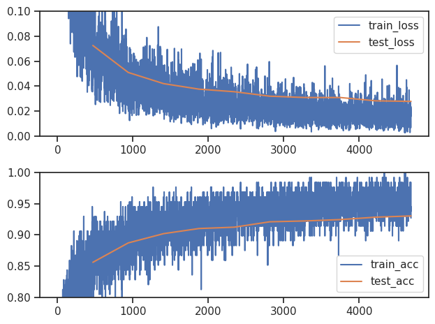
Finally we plot the learning curves
sns.set_theme("notebook")
sns.set_style("ticks")

iterations_per_epoch = len(train_dataloader)

fig, ax = plt.subplots(2, 1)
ax[0].plot(np.array(train_loss), label="train_loss")
ax[0].plot((np.arange(len(test_loss)) + 1) * iterations_per_epoch, np.array(test_loss).mean(-1), label="test_loss")
ax[0].set_ylim([0.0, 0.1])
ax[0].legend()

ax[1].plot(np.array(train_acc), label="train_acc")
ax[1].plot((np.arange(len(test_acc)) + 1) * iterations_per_epoch, np.array(test_acc).mean(-1), label="test_acc")
ax[1].set_ylim([0.8, 1.0])
ax[1].legend()

plt.tight_layout()
LSP decoupled the implementation of code editing features by allowing the implementation of a server which editors then used through a frontend. In this way the frontend implementation relies on a consistent API but does not actually have to reimplement the server for every editor.