Diffusion and score-based generative modeling
Diffusion and score-based generative modeling
There are great blog posts of what diffusion and score matching is elsewhere, in particular, see Lilian Weng's literature review and the great exposition of Yang Song on learning score functions for generative modeling. Here I will mainly lean on the blog post of Yang Song and his and his collaborators paper Generative Modeling by Estimating Gradients of the Data Distribution (Song and Ermon 2020) as I find it very comprehensive and well-written.
Some of the sections are pretty technical, for the actual implementation you only need to
- Read the Setup section,
- Understand how the loss \(\ell(\theta; \sigma)\) defined in \ref{eq:simplified-score-matching-objective} is used to build the optimization objective \(\hat{\mathcal{E}}(\theta; (\sigma_{l})_{l=1}^{L})\) defined in \ref{eq:aggregated-final-empirical-risk} which we train on to produce the estimator \(\hat{\theta}_{n}\) which are the learned parameters of the score network \(s_{\theta}\),
- Read the Generating samples section to understand how to generate samples using \(s_{\hat{\theta}_{n}}\),
and you should then be able to follow along with the implementation section.
Setup
To start with, we assume that we have a dataset of iid samples \((x_{i})_{i=1}^{n}\) sampled from some unknown data distribution \(p^{\ast}\), where the datapoints live in some space \(\mathcal{X}\) which we will take to be some Euclidean vector space (for example, \(\mathbb{R}^{D}\) for a vector or \(\mathbb{R}^{H \times W \times C}\) for an image with width \(W\), height \(H\) and \(C\) color channels). Everything is nice so we assume that \(p^{\ast}\) has a pdf and identify the distribution with this pdf (so \(p^{\ast}(x)\) is the density at \(x\)). The goal is to learn a model which would allow us to sample from \(p^{\ast}\). One way to do this would be to model \(p^{\ast}\) directly, but as fortune has it, it is enough to learn a model of the score function \(s^{\ast}(x) = \nabla_{x} \log p^{\ast}(x)\) to accomplish this.
Learning the score function using score matching allows for much easier training and modelling than trying to learn a model of \(p^{\ast}\) directly. This is due to not having to learn a properly normalized distribution but only up to a constant. If rewrite \(p^{\ast}(x) = \exp(-f^{\ast}(x))/Z^{\ast}\), the score function takes the form \(-\nabla_{x} f^{\ast}(x)\) since \[ \nabla_{x} \log p^{\ast}(x) = -\nabla_{x} f^{\ast}(x) - \nabla_{x}\log Z^{\ast} = -\nabla_{x} f^{\ast}(x) \] as \(Z^{\ast}\) is independent of \(x\).
Score matching
Score matching aim to minimize the least-squares objective
\begin{equation} \label{eq:lsq-score-matching-objective} \frac{1}{2}\mathbb{E}_{X \sim p^{\ast}}\|s_{\theta}(X) - s^{\ast}(X)\|^{2} \end{equation}where \(s_{\theta}: \mathcal{X} \to \mathcal{X}\) is a model of the score function, for example a neural network. Of course, we don't know \(s^{\ast}\) so this objective is not very good, but it can be shown to be proportional to
\begin{equation} \label{eq:tr-score-matching-objective} \mathbb{E}_{X \sim p^{\ast}}\left[\mathrm{tr}\left(\nabla_{x} s_{\theta}(X))\right) + \frac{1}{2}\|s_{\theta}(X)\|_{2}^{2}\right]. \end{equation}In practice, we replace the distribution \(p^{\ast}\) by the empirical version \(\hat{p}_{n}\) using the train dataset \((x_{i})_{i=1}^{n}\). When the input dimension is large the trace computation becomes too computational burdensome so we rely on other approximation. We will use denoising score matching, but there are other ways, in (Song and Ermon 2020) they also mention sliced score matching as an alternative.
To get to the point, denoising score matching replaces the distribution \(p^{\ast}\) with a smoothed version \(q_{\sigma}(x) = \mathbb{E}_{X' \sim p^{\ast}}\left[q_{\sigma}(x|X')\right]\) where \(q_{\sigma}\) is a some symmetric bell-curved distribution, for example a gaussian with standard deviation \(\sigma\) and mean \(X'\). Intuitively the scale parameter \(\sigma\) allow us to trade off some bias for variance by interpolating between the true (empirical) distribution as \(\sigma \to 0\) and a uniform distribution as \(\sigma \to \infty\)1, in addition to making training possible as it makes the resulting smoothed empirical distribution have full support on \(\mathcal{X}\) (so, it is never zero anywhere). Without this smoothing, \(\hat{p}_{n}\) will always be zero on points outside of the train set which comes with all kinds of problems. Choosing \(q_{\sigma}(x | x')\) to be an isotropic Gaussian pdf / distribution with covariance matrix \(\sigma I\) and mean \(x'\) simplifies objective \ref{eq:tr-score-matching-objective} to
\begin{equation} \label{eq:simplified-score-matching-objective} \mathcal{L}(\theta; \sigma) = \frac{1}{2}\mathbb{E}_{X \sim p^{\ast}}\mathbb{E}_{X' \sim q_{\sigma}(\cdot | X)}\left[\|s_{\theta}(X', \sigma) - (- (X' - X)/\sigma^{2})\|_{2}^{2}\right] \end{equation}where both the risk \(\mathcal{L}\) and the score model \(s_{\theta}\) are now indexed by \(\sigma\). We may think of this as parameterizing a family of score models by \(\sigma\) for some fixed \(\theta\). Let's call the empirical risk \(\ell(\theta; \sigma)\) where we replace \(p^{\ast}\) with the empirical distribution \(\hat{p}_{n}\). The final objective defining the Noise Conditional Score Network above average losses over a geometrically spaced grid of scales \(\sigma\). For such a grid \((\sigma_{l})_{l=1}^{L}\) we have
\begin{equation} \label{eq:aggregated-final-empirical-risk} \hat{\mathcal{E}}(\theta; (\sigma_{l})_{l=1}^{L}) = \frac{1}{L}\sum_{l=1}^{L}\lambda(\sigma_{l})\ell(\theta; \sigma_{l}) \end{equation}where \(\lambda\) is some weighing function which we will fix to be \(\lambda(\sigma) = \sigma^{2}\) according to the heuristic in (Song and Ermon 2020). Let us call the learned parameters \(\hat{\theta}_{n}\).
Generating samples
We can use Langevin dynamics to produce samples from the learned score model \(s_{\hat{\theta}_{n}}\). Usually, Langevin dynamics allow us to sample from some distribution \(p\) as long as we can evaluate the score function \(\nabla_{x} \log p(x)\). Fixing a step size (or more generally, a schedule) \(\eta\) and some prior distribution \(\pi\) we can sample an initial value \(x_{0}\) and iterate using
\begin{equation} \label{eq:langevin-dynamics} x_{t+1} = x_{t} + \frac{\eta}{2}\nabla_{x}\log p(x_{t}) + \sqrt{\eta}Z_{t} \end{equation}where \(Z_{t}\)'s are sampled iid from a unit Gaussian. Replacing \(\nabla_{x}\log p(x)\) with \(s_{\hat{\theta}_{n}}(x)\) we can generate samples hopefully resembling those from \(p^{\ast}\).
More generally, for any procedure which produces samples from a distribution \(p\) using only the score function, we can plug-in \(s_{\hat{\theta}_{n}}\) which we've learned and produce samples, using the plugin-estimator method. This is pretty nice, we can tap into all the work which has been done in the field of MCMC2, for example Hamiltonian Monte-Carlo or NUTS. The decoupling of training and inference leads to many benefits, as we can repurpose \(s_{\hat{\theta}_{n}}\) for other downstream tasks.
Implementation
Imports
import functools
import math

import matplotlib.pyplot as plt
import numpy as np
import seaborn as sns
sns.set_style("white")

import jax.numpy as jnp
from jax import grad, jax, vmap, lax
from jax import random
from jax import value_and_grad
import jax.tree_util as jtu
import jax

import equinox as eqx
import optax
from jaxtyping import Array, Float, Int, PyTree

import tensorflow_datasets as tfds
from tensorflow_probability.substrates import jax as tfp
tfd = tfp.distributions
tfb = tfp.bijectors
tfpk = tfp.math.psd_kernels
2024-02-05 13:35:57.262064: E external/local_xla/xla/stream_executor/cuda/cuda_dnn.cc:9261] Unable to register cuDNN factory: Attempting to register factory for plugin cuDNN when one has already been registered
2024-02-05 13:35:57.262106: E external/local_xla/xla/stream_executor/cuda/cuda_fft.cc:607] Unable to register cuFFT factory: Attempting to register factory for plugin cuFFT when one has already been registered
2024-02-05 13:35:57.263175: E external/local_xla/xla/stream_executor/cuda/cuda_blas.cc:1515] Unable to register cuBLAS factory: Attempting to register factory for plugin cuBLAS when one has already been registered
2024-02-05 13:35:58.023617: W tensorflow/compiler/tf2tensorrt/utils/py_utils.cc:38] TF-TRT Warning: Could not find TensorRT
Tractable mixture models
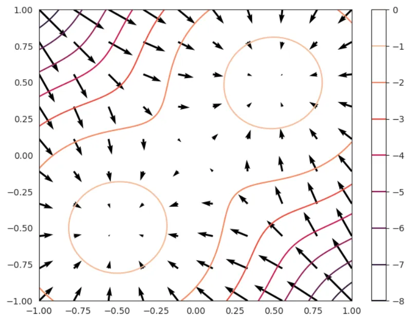
For some very simple models such as mixtures of tractable base models or using bijectors we don't even need to learn the score function since it's available to us in closed form. The simplest way to get some intuition for this is to visualize the the log-probability function \(\log p(x)\) using for example level-sets and the vector field corresponding to \(s(x)\) in 2 dimensions.
def plot_logdistribution(fig, ax, distribution, xlim=(-1.0, 1.0), ylim=(-1.0, 1.0), n_contour=100, n_quiver=10):
    # Define the grid for contour
    x = np.linspace(*xlim, n_contour)
    y = np.linspace(*ylim, n_contour)
    X, Y = np.meshgrid(x, y)
    XY = np.stack([X.ravel(), Y.ravel()], axis=-1)

    # Compute the log-distribution
    Z = distribution.log_prob(XY).reshape(n_contour, n_contour)
    cont = ax.contour(X, Y, Z)
    plt.colorbar(cont, ax=ax)

    # Compute the gradients
    x = np.linspace(*xlim, n_quiver)
    y = np.linspace(*ylim, n_quiver)
    X, Y = np.meshgrid(x, y)
    XY = np.stack([X.ravel(), Y.ravel()], axis=-1)
    grads = vmap(grad(distribution.log_prob))(XY)
    grad_X = grads[:, 0].reshape(n_quiver, n_quiver)
    grad_Y = grads[:, 1].reshape(n_quiver, n_quiver)
    ax.quiver(X, Y, grad_X, grad_Y)
    return fig, ax
We simply show the level sets and quiver plot (the vector field) of the log-distribution and the score function
key = random.PRNGKey(0)  # Use a different key for different runs

# Define a 2-component Gaussian Mixture model
num_components = 2
component_means = [(0.5, 0.5), (-0.5, -0.5)]
sd = 0.4
component_sds = [(sd, sd), (sd, sd)]
p1 = 0.5
component_probs = [p1, 1 - p1]

mixture_dist = tfd.Categorical(probs=component_probs)
component_dist = tfd.MultivariateNormalDiag(loc=component_means, scale_diag=component_sds)
mixture_model = tfd.MixtureSameFamily(
    mixture_distribution=mixture_dist,
    components_distribution=component_dist,
    name="MoG"
)

fig, ax = plt.subplots(figsize=(8, 6))
fig, ax = plot_logdistribution(fig, ax, mixture_model)
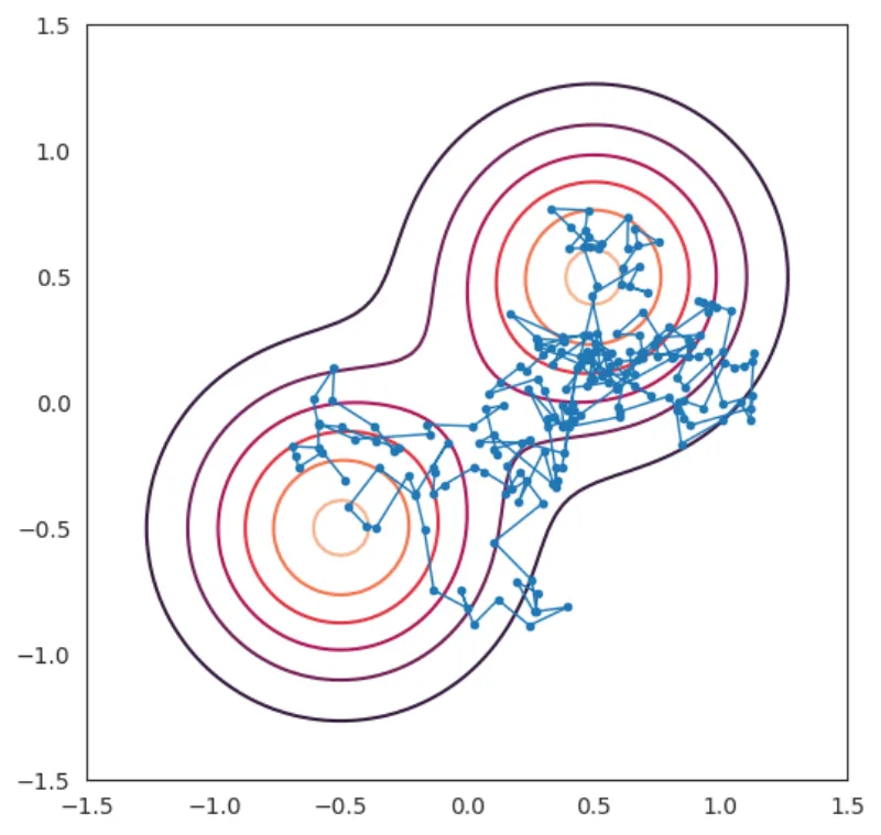
Generating samples
We already know from the previous section on generating samples how to do this, and the implementation is straightforward.
Let's quickly enable plotting the distribution. We will use this as a background for the evolving particle systems according to the Langevin dynamics.
def plot_distribution(fig, ax, distribution, xlim=(-1.0, 1.0), ylim=(1.0, 1.0), n_contour=100):
    # Define the grid for contour
    x = np.linspace(*xlim, n_contour)
    y = np.linspace(*ylim, n_contour)
    X, Y = np.meshgrid(x, y)
    XY = np.stack([X.ravel(), Y.ravel()], axis=-1)

    # Compute the distribution
    Z = distribution.prob(XY).reshape(n_contour, n_contour)
    cont = ax.contour(X, Y, Z)
    return fig, ax
We define the update step (return tuple due to using lax.scan later) and evolve a particle over many steps, lax.scan simply makes this efficient.
def update_x(x, z, distribution, step_size):
    g = grad(distribution.log_prob)(x)
    xp1 = x + (step_size / 2) * g + jnp.sqrt(step_size) * z
    return xp1, xp1

step_size = 0.01
num_steps = 200
key = random.PRNGKey(0)
z_key, x0_key, key = random.split(key, 3)
z = random.normal(z_key, shape=(num_steps, 2))
x0 = random.normal(x0_key, shape=(2,)) * 0.5
update_fun = functools.partial(update_x, distribution=mixture_model, step_size=step_size)
final, result = lax.scan(update_fun, x0, z)
Let's look at the result in this case. To see the path of the particle more clearly I'll outline the path by simply drawing a line between each point in result.
fig, ax = plt.subplots(figsize=(6, 6))
fig, ax = plot_distribution(fig, ax, mixture_model, xlim=(-1.5, 1.5), ylim=(-1.5, 1.5))
ax.plot(result[:, 0], result[:, 1], marker=".", linewidth=1.0)
Finally, let's make a video for goodies. The video is the above plot shown in time, following the particle according to the Langevin dynamics.
# We will animate this using the FuncAnimation class from matplotlib
from matplotlib.animation import FuncAnimation
fig, ax = plt.subplots(figsize=(6, 6))
fig, ax = plot_distribution(fig, ax, mixture_model, xlim=(-1.5, 1.5), ylim=(-1.5, 1.5))

# Initialize the line plot
line, = ax.plot([], [], marker='.', linewidth=1.0)
# Initialize the particle positions
positions = result

# Function to update the line plot
def update(frame):
    # Update the line plot data
    line.set_data(positions[:frame+1, 0], positions[:frame+1, 1])
    return line,

# Create the FuncAnimation
animation = FuncAnimation(fig, update, frames=len(positions),
                          interval=100, repeat=False)

# Save using ffmpeg
animation.save("mog-langevin-dynamics.mp4", writer="ffmpeg", dpi=200)
Learning the score function
The reason we didn't have to learn the score function in Tractable mixture models was because we restricted ourselves to a distribution with a tractable score function. In reality this is seldom the case, and even if we could do it in theory, it may be too computationally expensive to do it directly. Additionally, If we have a set of points which we interpret as an empirical distribution then the score function is not even well-defined as there is no density. We have to resort to learning it in some way.
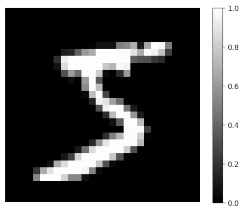
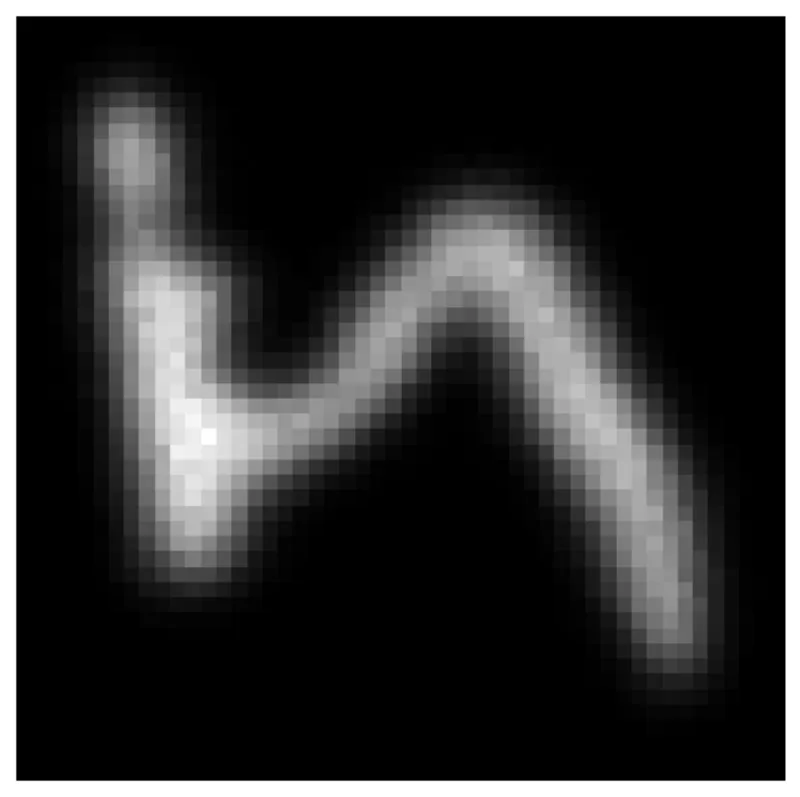
First, we will use the MNIST dataset where we view an image as a discrete distribution by normalizing the pixel intensities over the total intensity of all the pixels in the image. Since each pixel is a value between 0 and 1, we can view this as a distribution over pixel coordinates. To make this point clear, we assume that the underlying space is a 2d cartesian square, \(\mathcal{X} = [0, 1]^{2}\)3, with each pixel coordinate being normalized to be between 0 and 1. So, an image is a collection of coordinate pairs and pixel intensity values, in the case of MNIST which is \(28 \times 28\) we have pixel coordinates \((i, j)\) where \(i, j \in \{(l + 1/2) / 28\}_{l=0}^{27}\) and the corresponding pixel intensities \(I(i, j) \in [0, 1]\). With this we have an empirical distribution where \(\hat{p}(i, j) = I(i, j) / \sum_{i', j'}I(i', j') \propto I(i, j)\).
Behold, the first image to the MNIST training dataset!
# Get an image from mnist
import torchvision

mnist = torchvision.datasets.MNIST("~/data", download=True)
mnist_images = mnist.data.numpy()
image = mnist_images[0]
image = image.astype(float) / 255.0

def create_sample_fn(image):
    """Generate a function that samples from the image distribution"""
    def sample(num_samples, key):
        h, w = image.shape
        # Note that random.categorical takes as inputs logits which is why we do not have to normalize
        return jnp.array(
            [divmod(x.item(), w) for x in random.categorical(logits=jnp.log(image.ravel()), key=key, shape=(num_samples,))]
        )
    return sample

fig, ax = plt.subplots()
im = ax.imshow(image, cmap="gray")
plt.colorbar(im)
ax.axis("off")
Let's check the histogram when we sample many times according to the distribution defined by the image, we should get something similar as the sample size becomes large. The histogram function will rotate the image though.
key = jax.random.PRNGKey(sum(ord(c) for c in "five"))
sample = create_sample_fn(image)
x = sample(10000, key)
fig, ax = plt.subplots(figsize=(4, 4))
h = ax.hist2d(x[:, 0], x[:, 1], cmap="gray")
ax.axis("off")

Now we set up the training. The architecture here is a combination of things
- We use the insights from (Tancik et al. 2020) which roughly says that using a pre-processing fourier feature map before the MLP is helpful for learning high-frequency mappings for coordinate based inputs. We add a residual connection here, so that the input to the MLP is jnp.concatenate(f_layer(x), x).
- The RFLayer has noise-level specific parameters alpha, beta which linearly transform the random features and we learn one such transformation for each noise level (the rest of the architecture is shared, like the MLP and the original random feature mappings).
- We freeze the random feature parameters B_cos, B_sin by following the guide on how to freeze layer in the equinox documents.
- The rest of the training is done using the objective \(\hat{\mathcal{E}}(\theta; (\sigma_{l})_{l=1}^{L})\).
class RFLayer(eqx.Module):
    """Random Feature layer with learnable linear output transformations alpha, beta"""
    B_cos: jax.Array
    B_sin: jax.Array
    alpha: jax.Array
    beta: jax.Array
    num_noise_levels: int
    sigma: float

    def __init__(self, in_size: int, num_rf: int, num_noise_levels: int, key, sigma: float = 1.0):
        cos_key, sin_key = random.split(key, 2)
        self.B_cos = random.normal(cos_key, (num_rf, in_size)) * sigma
        self.B_sin = random.normal(sin_key, (num_rf, in_size)) * sigma
        self.sigma = sigma
        self.num_noise_levels = num_noise_levels
        self.alpha = jnp.ones(num_noise_levels)
        self.beta = jnp.zeros(num_noise_levels)

    def __call__(self, x: jax.Array, noise_level_idx: int) -> jax.Array:
        rf_features = jnp.concatenate(
            [jnp.cos(2 * math.pi * self.B_cos @ x), jnp.sin(2 * math.pi * self.B_sin @ x)], axis=-1
        )
        return self.alpha[noise_level_idx] * rf_features + self.beta[noise_level_idx]

class Model(eqx.Module):
    rf_layer: RFLayer
    mlp: eqx.nn.MLP

    def __init__(self, in_size: int, num_rf: int, width_size: int, depth: int, out_size: int, num_noise_levels: int, key):
        self.rf_layer = RFLayer(in_size, num_rf, num_noise_levels, key)
        self.mlp = eqx.nn.MLP(in_size=num_rf * 2 + 2,
                              width_size=width_size,
                              depth=depth,
                              out_size=out_size,
                              activation=jax.nn.softplus,
                              key=key)

    def __call__(self, x: jax.Array, noise_level_idx: int) -> jax.Array:
        x -= 0.5
        x = jnp.concatenate((self.rf_layer(x, noise_level_idx), x)) #Residual connection
        return self.mlp(x)

# Define the objective function
def one_sample_loss(model, x, sigmas, key):
    # Sample one gaussian for each noise level
    perturbations = random.normal(key, (sigmas.shape[0], x.shape[0])) * jnp.expand_dims(sigmas, 1)
    x_bars = x + perturbations
    # Predict over all noise levels
    scores_pred = vmap(model)(x_bars, jnp.arange(sigmas.shape[0]))
    scores = -(x_bars - x) / jnp.expand_dims(sigmas ** 2, 1)
    # Vectorized version of (x_bar[i] - x) / sigma[i] ** 2
    # mean(sigmas[i]**2 * mse(score_pred[i], scores[i]) for i in range(len(sigmas))))
    result = jnp.mean(jnp.square(scores_pred - scores).mean(-1) * sigmas ** 2)
    return result

def loss(diff_model, static_model, xs, sigmas, keys):
    """Objective function, we separeate the parameters into active and frozen parameters"""
    model = eqx.combine(static_model, diff_model)
    batch_loss = vmap(one_sample_loss, (None, 0, None, 0))
    return jnp.mean(batch_loss(model, xs, sigmas, keys))

def train(
        model: eqx.Module,
        filter_spec: PyTree,
        sample,
        optim: optax.GradientTransformation,
        steps: int,
        batch_size: int,
        print_every: int,
        sigmas: Float[Array, "..."],
        key
) -> eqx.Module:
    @eqx.filter_jit
    def make_step(
            model: eqx.Module,
            xs: Float[Array, "batch_size 2"],
            opt_state: PyTree,
            keys: Float[Array, "batch_size"],
    ):
        diff_model, static_model = eqx.partition(model, filter_spec)
        loss_value, grads = eqx.filter_value_and_grad(loss)(diff_model, static_model, xs, sigmas, keys)
        updates, opt_state = optim.update(grads, opt_state)
        model = eqx.apply_updates(model, updates)
        return model, opt_state, loss_value

    original_model = model
    opt_state = optim.init(eqx.filter(model, eqx.is_inexact_array))
    for step in range(steps):
        *loss_keys, sample_key, key = random.split(key, batch_size + 2)
        loss_keys = jnp.stack(loss_keys)
        xs = sample(batch_size, sample_key) / 27
        model, opt_state, loss_value = make_step(model, xs, opt_state, loss_keys)
        if step % print_every == 0:
            print(f"Step {step}, Loss {loss_value}")

    return model
Now let's train it. We squint and choose some good hyperparameters and pray to the ML-gods for an auspicious training run (actually I did some hand-tuning).
sigmas = jnp.geomspace(0.0001, 1, 30, endpoint=True)
DEPTH = 3
WIDTH_SIZE = 128
NUM_RF = 256
BATCH_SIZE = 128
STEPS = 5 * 10 ** 4
PRINT_EVERY = 5000

model = Model(in_size=2,
              num_rf=NUM_RF,
              width_size=WIDTH_SIZE,
              depth=DEPTH,
              out_size=2,
              num_noise_levels=len(sigmas),
              key=random.PRNGKey(0))

LEARNING_RATE = 1e-3
optim = optax.adam(LEARNING_RATE)

# The filter spec is a pytree of the same shape as the parameters
# True and False represent whether this part of the pytree will be updated
# using the optimizer by splitting the parameters into diff_model and static_model
filter_spec = jtu.tree_map(lambda x: True if isinstance(x, jax.Array) else False, model)
filter_spec = eqx.tree_at(
    lambda tree: (tree.rf_layer.B_cos, tree.rf_layer.B_sin),
    filter_spec,
    replace=(False, False),
)
model = train(model, filter_spec, sample, optim, STEPS, BATCH_SIZE, PRINT_EVERY, sigmas, key)
Step 0, Loss 1.0177688598632812
Step 5000, Loss 0.7470076084136963
Step 10000, Loss 0.6700457334518433
Step 15000, Loss 0.6010410785675049
Step 20000, Loss 0.5470178127288818
Step 25000, Loss 0.5063308477401733
Step 30000, Loss 0.47549256682395935
Step 35000, Loss 0.4591177701950073
Step 40000, Loss 0.4523712992668152
Step 45000, Loss 0.43943890929222107
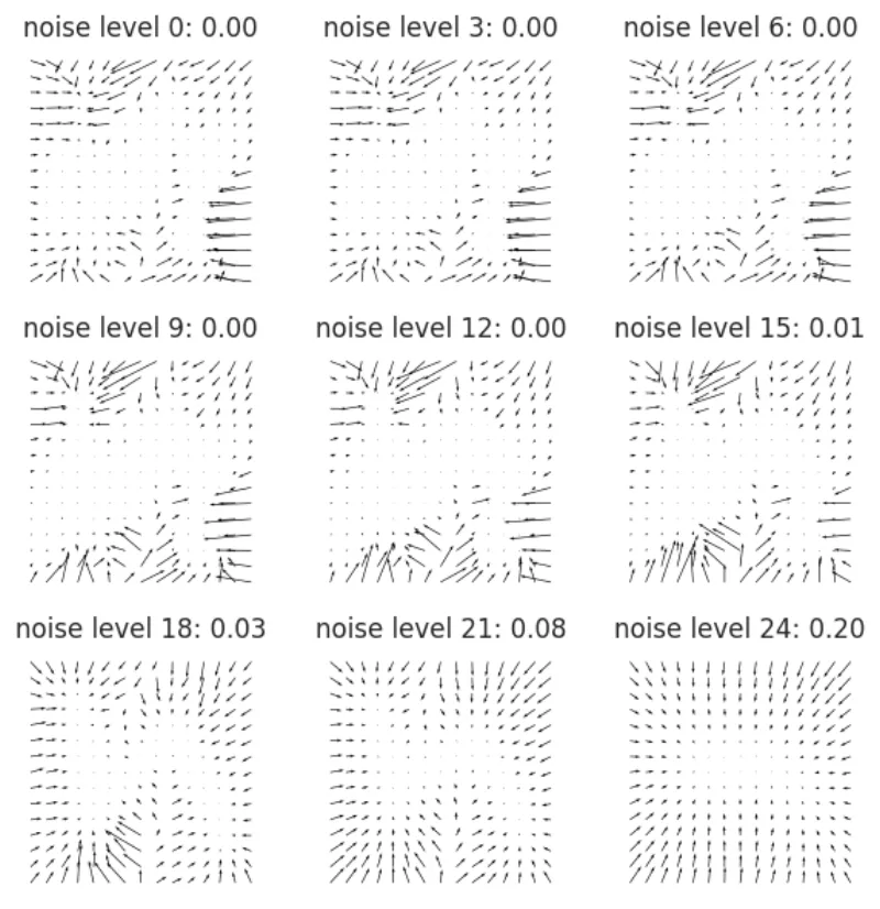
Let's visualize the vector field for this new model by repurposing the plot_logdistribution function to just plot the vector field. Since we don't have an actual density we will not plot the level
def plot_vector_field(fig, ax, score_fun, xlim=(0.0, 1.0), ylim=(0.0, 1.0), n_quiver=10):
    # Compute the gradients
    x = np.linspace(*xlim, n_quiver)
    y = np.linspace(*ylim, n_quiver)
    X, Y = np.meshgrid(x, y)
    XY = np.stack([X.ravel(), Y.ravel()], axis=-1)
    grads = vmap(score_fun)(XY)
    grad_X = grads[:, 0].reshape(n_quiver, n_quiver)
    grad_Y = grads[:, 1].reshape(n_quiver, n_quiver)
    ax.quiver(X, Y, grad_X, grad_Y)
    return fig, ax

fig, ax = plt.subplots(3, 3, figsize=(3 * 2, 3 * 2))
for axis, i in zip(ax.ravel(), range(0, 30, 3)):
    axis.axis('off')
    axis.set_aspect('equal')
    axis.set_title(f"noise level {i}: {sigmas[i]:.2f}")
    plot_vector_field(fig, axis, functools.partial(model, noise_level_idx=i), n_quiver=15)

plt.tight_layout()
Let's see what we have learned. We define the update step (return tuple due to using lax.scan later)
@eqx.filter_jit
def update_x(x, z, model, step_size):
    g = model(x)
    xp1 = x + (step_size / 2) * g + jnp.sqrt(step_size) * z
    return xp1, xp1
and evolve a particle over many steps, lax.scan simply makes this efficient
step_size = 0.001
num_steps = 400_000
key = random.PRNGKey(0)
z_key, x0_key, key = random.split(key, 3)
z = random.normal(z_key, shape=(num_steps, 2))
x0 = jnp.ones(2,) * 0.5
score_model = functools.partial(model, noise_level_idx=17)
update_fun = functools.partial(update_x, model=score_model, step_size=step_size)
final, result = lax.scan(update_fun, x0, z)
Let's look at this. Since we sample so many particles, let's just plot a 2d histogram of this (choosing noise_level_idx being 17 but other indices in the vicinity should work too). Note that this has a finer resolution than the original mnist images which are \(27 \times 27\)
fig, ax = plt.subplots(figsize=(6, 6))
h = ax.hist2d(result[:, 0], result[:, 1], cmap="gray", bins=(50, 50))
ax.axis("off")
Conclusion
This was a great way to learn jax and how diffusion works. Looking back I think it may be overkill to do this on images as distributions as I did above, learning the distribution directly may be better in this case and faster in this case. I like the fact that the score model generalizes from the grid points \((i/27, j/27)_{i, j}^{27}\) to any tuple of points \((i, j)_{i, j \in [0, 1]}\) which is pretty cool and makes me wonder if you can use this to create a way to combine images of different resolutions as long as the aspect ratio is the same.
Reference
Feels like there should be some way of looking at this through a regularization lense where \(\sigma\) takes the role as the regularization strength in traditional supervised learning such as Ridge Regression.
Of which I know very little.
Although when we convolve the inputs with Gaussians we will have that any point in \(\mathbb{R}^{2}\) will have positive probability, albeit maybe very small.